Classification
In many cases we may encounter data which contain categorical variables instead of quantitative variables. An example of categorical data could be something like a dataset containing a coloumn of a variable called “Eye Colour” with entries such as “Blue” or “Brown” instead of numerical values. In some cases we could decide to convert categorical data to numerical data if the assignment is appropriate. For example if there are only two possible options we can map one choice to the number 1 and the alternative to the number 0. An example would be a column called “Passed” with entries being either “Yes” or “No”, and we can map each “Yes” to 1 and each “No” to 0.
In general we use classification to predict qualitative responses for categorical data. To extract direct meaning from the term “Classification”: We classify an observation and assign it to a category. There are many classification techniques, some of the more popular ones are logistic regression, linear and quadratic discriminant analysis, naive Bayes and K-nearest neighbours.
1. Logistic Regression
Let’s go back to the example where we have a column called “Passed” which contains data labeled either “Yes” or “No”. This could be a column containing data on whether a student has passed a course, and it is clear that a response can fall into one of two categories. Logistic regression is a reasonable model for a situation like this where we encounter a binary outcome. The logistic regression models the probability that the response $Y$ belongs to one of the categories based on some independent value. In this case the logistic regression model would return the probability of a pass based on a student’s overall course grade, so we would have $Pr(\text{pass}|\text{grade})$.
So in general, the logistic regression model can be expressed as
$p(X)=Pr(Y=1|X)=\dfrac{e^{\beta_{0}+\beta_{1}X}}{1+e^{\beta_{0}+\beta_{1}X}}$
This model (i.e. the parameters $\beta_{0}, \beta_{1}$) can be fitted with the maximum likelihood method. The estimates $\widehat\beta_{0}$ and $\widehat\beta_{1}$ should maximise the likelihood function $l(\beta_{0}, \beta_{1})$ given by
$l(\beta_{0}, \beta_{1})=\displaystyle{\prod_{i:y_{i}=1}p(x_{i})\prod_{i’:y_{i’}=0}(1-p(x_{i’}))}$
We can start making predictions once the coefficients have been estimated by using
$\widehat{p}(X)=\widehat{Pr}(Y=1|X)=\dfrac{e^{\widehat\beta_{0}+\widehat\beta_{1}X}}{1+e^{\widehat\beta_{0}+\widehat\beta_{1}X}}$
which returns a value between 0 and 1. Now suppose we add more predictors such as class attendance, hours studies etc, then we will have to use a multiple logistic regression model for $p$ predictors which is simply
$p(X)=Pr(Y=1|X)=\dfrac{e^{\beta_{0}+ \beta_{1}X_{1} + … + \beta_{p}X_{p}}}{1+e^{\beta_{0}+ \beta_{1}X_{1} + … + \beta_{p}X_{p}}}$
Dataset Description
Our task is to create a model that predicts whether a student will pass a particular course based on their final score. This is a trivial application since it is easy to see that a student will pass (Y=1) given that the student’s score is greater than the passing score, so P(Y=1 | x=0.5) = 1 is a reasonable model in this case. We start by constructing the dataset.
# Import necessary libraries
import numpy as np
import pandas as pd
import matplotlib.pyplot as plt
import seaborn as sn
import statsmodels.api as sm
from sklearn.model_selection import train_test_split
from sklearn.linear_model import LogisticRegression
from sklearn import metrics

# Set a numpy seed for reproducibility
np.random.seed(0)

# Generate random student scores for 100 students
scores = np.random.randint(0, 101, 100)

# Create a dataframe containing the scores
df = pd.DataFrame({'Score' : scores})

# Create a pass column containing categorical labels based on the score column
df['Pass'] = np.where(df['Score'] >= 50, 'Yes', 'No')

# Display the first five entries
display(df.head())
| Score | Pass | |
|---|---|---|
| 0 | 44 | No |
| 1 | 47 | No |
| 2 | 64 | Yes |
| 3 | 67 | Yes |
| 4 | 67 | Yes |
Data Cleaning
Since we have created the dataset, the dataset is already cleaned, however we still have to convert the categorical data contained in the ‘Pass’ column to binary values.
# Convert categorical data to binary values
df['Pass'] = (df['Pass'] == 'Yes').astype(int)

# Display new dataframe
display(df.head())
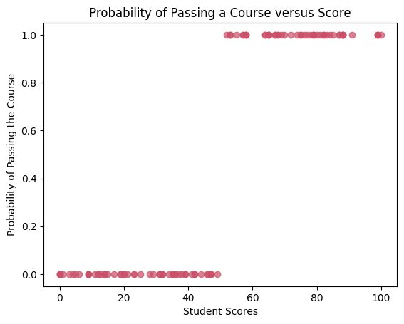
Data Visualisation
Next we create a scatter plot of the data.
# Define X data
X = df[['Score']]

# Define Y Data
Y = df[['Pass']]

# Plot the data
plt.plot(X, Y, 'o', color='#CA4F67', alpha=0.7)
plt.title('Probability of Passing a Course versus Score')
plt.xlabel('Student Scores')
plt.ylabel('Probability of Passing the Course')
plt.show()
Training the Model
Next we split the data into training and testing data and fit the logistic regression model.
# Split the data
X_train, X_test, y_train, y_test = train_test_split(X, Y, test_size=0.20, random_state=1)

# Create a logistic regression object
logistic_regression = LogisticRegression()

# Pass the data through the model
logistic_regression.fit(X_train, y_train)

# Make predictions
y_predicted = logistic_regression.predict(X_test)
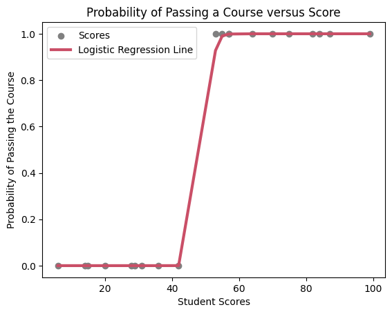
Results
# Get probabilities
y_probability = logistic_regression.predict_proba(X_test)[:, 1]

# Plot the results
plt.scatter(X_test, y_test, color='gray', label='Scores')
plt.plot(np.sort(X_test.values.ravel()), np.sort(y_probability), color='#CA4F67', linewidth=3, linestyle='-', label="Logistic Regression Line")
plt.legend()
plt.title('Probability of Passing a Course versus Score')
plt.xlabel('Student Scores')
plt.ylabel('Probability of Passing the Course')
plt.show()

# Display model accuracy
display(f'Model Accuracy: {metrics.accuracy_score(y_test, y_predicted) * 100}%')
'Model Accuracy: 100.0%'
We see that in this simple test case the model made predictions with an accuracy of 100%. However this is due to the simplicity of the data.